Python Image Read and Get Rgb Channels

Introduction to Image Processing with Python — Colour Channel Histogram Manipulation for Beginners

How to perform histogram manipulation for each color channel in your image.

RGB Adjusted Bookstore (Image by Author)

Previously, I wrote an article regarding Histogram Manipulation. In it I discussed the nuts of adjusting grayscale image values to make the overall prototype more palatable for humans. I briefly touched on the idea of adjusting the Cumulative Distribution Part for colored images, but stopped brusque of discussing the best way to practise it. In this article nosotros shall tackle just that.

Let's get started!

As per usual, allow united states first import all the required libraries.

          import numpy as np
import matplotlib.pyplot as plt
from skimage.io import imread, imshow
import matplotlib.pyplot as plt
from skimage.exposure import histogram, cumulative_distribution
from skimage import img_as_ubyte, img_as_float
from scipy.stats import norm        

Smashing! Now let us load the image.

          dark_image = imread('dark_books.png');
plt.figure(num=None, figsize=(8, 6), dpi=80)
imshow(dark_image);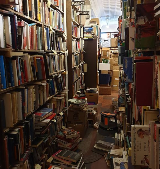        

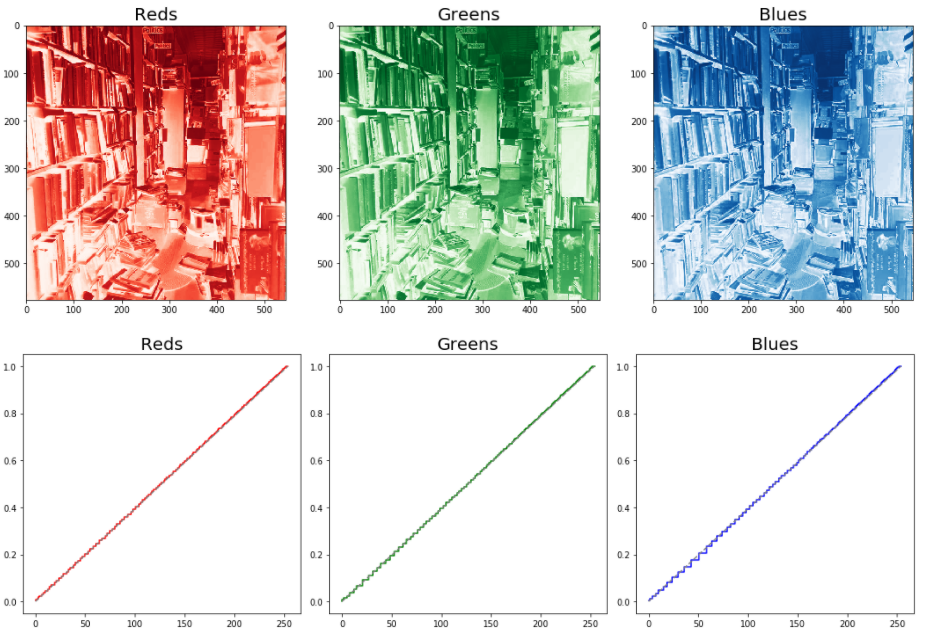
Dark Books (Image by Author)

To help us get a b etter idea of the RGB layers in this prototype, allow united states of america segregate each individual channel. Below is a useful code that will do that for whatever image.

          def rgb_splitter(prototype):
            rgb_list = ['Reds','Greens','Blues']
            fig, ax = plt.subplots(1, 3, figsize=(17,7), sharey = True)
            for i in range(3):
            ax[i].imshow(image[:,:,i], cmap = rgb_list[i])
            ax[i].set_title(rgb_list[i], fontsize = 22)
            ax[i].axis('off')
            fig.tight_layout()          rgb_splitter(dark_image)        

RGB Channels of the Prototype

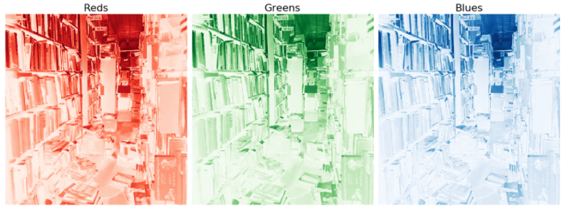
Nice! We now accept a general idea of what the individual color channels look like. Let us now cheque their CDFs, beneath is a useful office which will aid the states.

          def df_plotter(image):
            freq_bins = [cumulative_distribution(image[:,:,i]) for i in
            range(iii)]
            target_bins = np.arange(255)
            target_freq = np.linspace(0, one, len(target_bins))
            names = ['Red', 'Greenish', 'Blue']
            line_color = ['red','green','blue']
            f_size = xx
                  fig, ax = plt.subplots(1, 3, figsize=(17,5))
              for n, ax in enumerate(ax.flatten()):
              ax.set_title(f'{names[northward]}', fontsize = f_size)
              ax.pace(freq_bins[n][1], freq_bins[n][0], c=line_color[n],
              characterization='Bodily CDF')
              ax.plot(target_bins,              
              target_freq,              
              c='gray',              
              label='Target CDF',
              linestyle = '--')
                    df_plotter(dark_image)        

CDFs of the RGB Channels

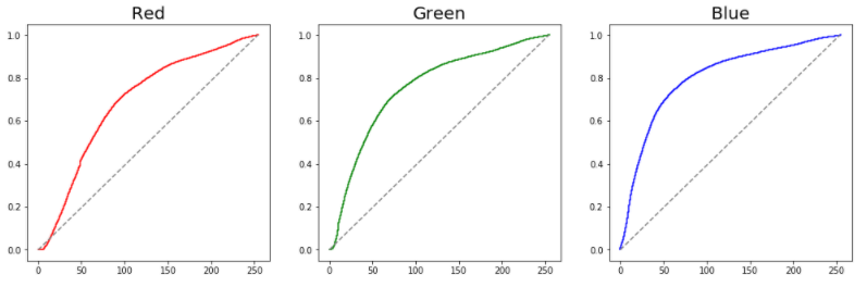
As we can see, all three channels are quite far from the arcadian straight line. To gear up that let the states simply interpolate their CDFs. Again, below is a useful function that does that for us.

          def rgb_adjuster_lin(image):
                  target_bins = np.arange(255)
              target_freq = np.linspace(0, one, len(target_bins))
              freq_bins = [cumulative_distribution(image[:,:,i]) for i in              
              range(iii)]
              names = ['Reds', 'Greens', 'Blues']
              line_color = ['red','dark-green','blue']
              adjusted_figures = []
              f_size = 20
            
                  fig, ax = plt.subplots(1,3, figsize=[15,5])
              for north, ax in enumerate(ax.flatten()):
              interpolation = np.interp(freq_bins[n][0], target_freq,              
              target_bins)
              adjusted_image = img_as_ubyte(interpolation[image[:,:,              
              n]].astype(int))
              ax.set_title(f'{names[north]}', fontsize = f_size)
              ax.imshow(adjusted_image, cmap = names[northward])
              adjusted_figures.append([adjusted_image])
                                fig.tight_layout()                      fig, ax = plt.subplots(ane,3, figsize=[fifteen,v])
            for n, ax in enumerate(ax.flatten()):
            interpolation = np.interp(freq_bins[n][0], target_freq,            
            target_bins)
            adjusted_image = img_as_ubyte(interpolation[prototype[:,:,            
            n]].astype(int))
            freq_adj, bins_adj = cumulative_distribution(adjusted_image)
                      ax.set_title(f'{names[due north]}', fontsize = f_size)
              ax.step(bins_adj, freq_adj, c=line_color[n], label='Actual              
              CDF')
              ax.plot(target_bins,              
              target_freq,              
              c='grayness',              
              characterization='Target CDF',
              linestyle = '--')
              fig.tight_layout()
              return adjusted_figures
                    channel_figures = return adjusted_figures        

Color Adjusted Images

We see meaning comeback per color channel, with all of them about resembling a directly line.

Additionally, note how this function returns all these values every bit a listing of lists. This volition serves us well for our final step, putting information technology all back together into a single moving-picture show. To give usa a improve thought of how this tin exist done, let us audit our list of lists.

          print(channel_figures)
impress(f'Total Inner Lists : {len(channel_figures)}')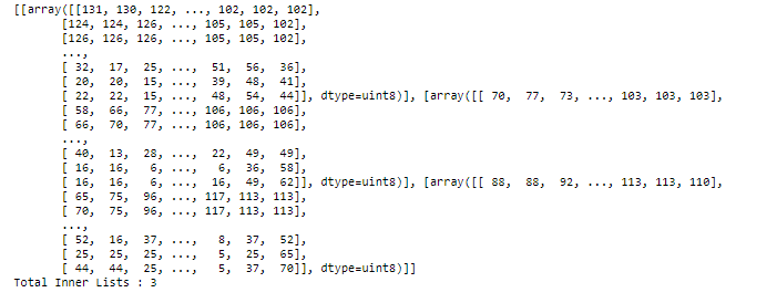        

Contents of channel_figures

We see that within the variable channel_figures are three lists. These lists represent the values for the RGB channel. This being the case, it is possible for united states to stitch all these values dorsum together. The below lawmaking does just that.

          plt.effigy(num=None, figsize=(10, 8), dpi=lxxx)
imshow(np.dstack((channel_figures[0][0],            
            channel_figures[ane][0],            
            channel_figures[2][0])));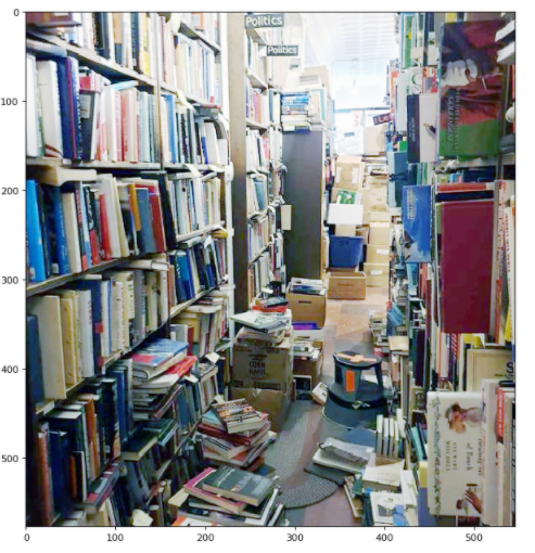        

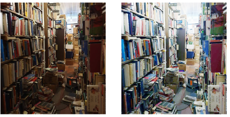
Reconstructed Colored Bookstore Image

Note how significant the difference is. Not only does the image seem significantly brighter, the xanthous clouded was also removed. Allow us try this aforementioned technique on a unlike epitome. Fortunately we accept already laid virtually of the groundwork by setting upwardly function. The below is just plug and play.

          dark_street = imread('dark_street.png');
plt.figure(num=None, figsize=(8, half-dozen), dpi=80)
imshow(dark_street);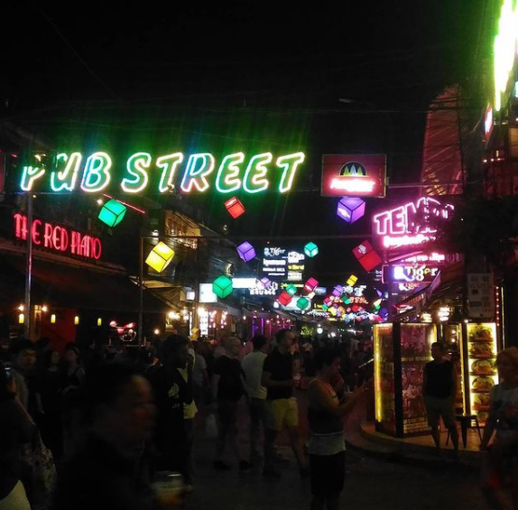        

Night Street (Image by Writer)

Now that nosotros have loaded our new picture, let united states of america simply run it by our functions.

          channel_figures_street = adjusted_image_data = rgb_adjuster_lin(dark_street)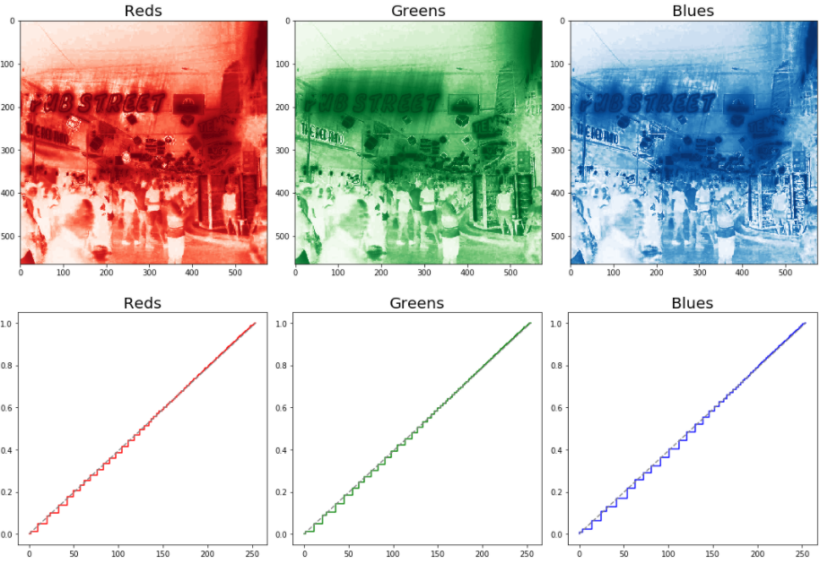        

Color Adjusted Images

          plt.effigy(num=None, figsize=(10, 8), dpi=80)
imshow(np.dstack((channel_figures_street [0][0],            
            channel_figures_street [one][0],            
            channel_figures_street [two][0])));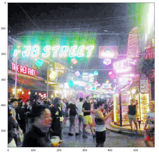        

Reconstructed Colored Street Image

Nosotros tin see an astonishing comeback. Though admittedly the image is slightly overexposed. This may be due to the significantly vivid neon lights in the back. In futurity articles, we shall learn how to fine tune our adjustment methodologies then that our functions can be more generalizable.

In Decision

In this article we learned how to suit each RGB aqueduct to preserve the color information of the prototype. Such a technique is a corking comeback over the previous grayscale adjustment method. Going frontwards we will discuss the many different distributions i can snap the CDF into. Such fine tuning of the adjustment methodology should help us better our functions then that they tin can piece of work with whatsoever image.

I know that this particular commodity has been quite function heavy, and for many beginners this may be a challenge to sympathise. Hopefully, yous can get the hang of using functions as they make working with Python a much more than efficient (and dare I say fun) activity.

cummingschmervaske1954.blogspot.com

Source: https://towardsdatascience.com/introduction-to-image-processing-with-python-color-channel-histogram-manipulation-for-beginners-d1d77dcb998d

Share this post